Modeling Tips
Applying In-Plane Moment to Plates
Occasionally you
may need to model an applied in-plane moment at a
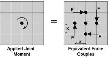
This might require re-meshing the area
receiving the moment into smaller plates so that the load area can be
more accurately modeled. If a beam member is attached to the
Modeling a Beam Fixed to a Shear Wall
Occasionally you
may need to model the situation where you have a beam element that is
fixed into a shear wall. A situation where this may occur would
be a concrete beam that was cast integrally with the shear wall or a steel
beam that was cast into the shear wall. The beam cannot just be
attached to the
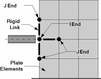
The only trick
to this method is getting the proper member end releases for the rigid
links. We want to transfer shear forces from the wall
Modeling a Cable
While there is not a true “cable element”, there is a tension only element. A true cable element will include the effects of axial pre-stress as well as large deflection theory, such that the flexural stiffness of the cable will be a function of the axial force in the cable. In other words, for a true cable element the axial force will be applied to the deflected shape of the cable instead of being applied to the initial (undeflected) shape. If you try to model a cable element by just using members with very weak Iyy and Izz properties and then applying a transverse load, you will not get cable action. What will happen is that the beam elements will deflect enormously with NO increase in axial force. This is because the change in geometry due to the transverse loading will occur after all the loads are applied, so none of the load will be converted into an axial force.
Guyed Structure (“Straight” Cables)
You can easily model cables that are straight and effectively experience only axial loading. If the cable is not straight or experiences force other than axial force then see the next section.
When modeling guyed structures you can model the cables with a weightless material so that the transverse cable member deflections are not reported. If you do this you should place all of the cable self-weight elsewhere on the structure as a point load. If you do not do this then the cable deflections (other than the axial deflection) will be reported as very large since it is cable action that keeps a guyed cable straight. If you are interested in the deflection of the cable the calculation is a function of the length and the force and you would have to calculate this by hand.
The section set for the cable; should be modeled as a tension only member so that the cable is not allowed to take compression. See T/C Members for more on this.
To prestress the cable you can apply a thermal load to create the pre-tension of the cable. See Prestressing with Thermal Loads to learn how to do this.
Modeling Composite Behavior
Occasionally you may want to model a structure with composite behavior. A practical situation where this arises is with composite concrete floor slabs, which have concrete slabs over steel or concrete beams. Another common case where composite behavior may be considered is where you have a steel tank with stiffeners. The stiffeners might be single angles or WT shapes.
The most accurate way to model this behavior for composite floor systems is to use a program (such a RISAFloor) that was created explicitly for this purpose. If that is not an option you may want to use an arbitrary member with an effective moment of inertia, Ieff, calculated according to the AISC or Canadian code provisions. This method has the advantage of being able to account for the effects of partial composite behavior, while the methods described below assume perfect connectivity between the steel beam and the concrete slab.
If you have already modeled the concrete
deck with plate elements, then the situation can be quickly modeled for
horizontal beams by using one beam modeled as a physical member and also
using Analysis Offsets. The beam would simply be drawn along the plates/
An example of a plate/beam model with composite action included using rigid links is shown here:
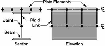
Note that beams and plates are each modeled at their respective centerlines. It is this offset of the beam and plate centerlines that causes the composite behavior. The distance between the centerlines is typically half the depth of the beam plus half the thickness of the plate elements. If the beam is an unsymmetrical shape, like a WT about the z-z axis or a single angle, then you would use the distance from the flange face to the neutral axis.
As shown above, a
rigid link is used to connect each set of
Graphical editing offers the fastest way
to model composite action. It is usually best to model the plates
with an appropriately fine mesh first. Then you would copy the plate
There are a number
of ways to build your rigid link member between all the corresponding
plate and beam
Now perform a model
merge. If you have used finite members rather than Physical Members
the merge Model Merge will break up finite element beams at all the intermediate
locations. See Model
Merge for more information. If you’re using physical members,
performing the model merge will clean up duplicate
Modeling Inclined Supports
You can model inclined supports by
using a short rigid link to span between a
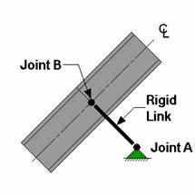
The rigid link should be “short”, say no more than 0.1 ft. The
member end releases for the rigid link at
The section forces in the rigid link
are the inclined reactions. Note that you need to make sure
the rigid link is connected to the members/plates at the correct inclined
angle. You can control the incline of the angle using the coordinates
of
Modeling One Member Over Another
Occasionally you may need to model the situation where one member crosses over another member. A common situation where this occurs is in the design of framing for crane rails, where the crane rail sits on top of, or is hanging beneath, the supporting beam. See the figure below:
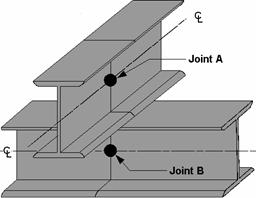
The two beams are each modeled at their
correct centerline elevations. Both the top and bottom members need
to have a
Reactions at Nodes with Enforced Displacements
The reaction at an enforced displacement can
be obtained by inserting a very short (.02' or so) rigid link between
the
Rigid Links
Rigid links are used to rigidly
transfer the forces from one point to another and to also account for
any secondary moments that may occur due to moving the force. This
is in contrast to using the tether feature for
Make a Rigid Link
To make a Rigid Link:
-
On the General tab of the Materials spreadsheet:
-
Create a material Label called “LINK”.
-
Enter “1e6 (ksi)” for the value of E.
-
Blank out the value for G by going to that column and pressing the space bar.
-
Double check that the Density is set to zero.
-
Leave all the other values as their defaults.
-
-
On the General tab of the Section Sets spreadsheet, create a section set Label called “RIGID” with the “LINK”Material.
- Move the cursor to the Shape column and hit your space bar to erase the information in this field.
- Set the A,and Iy, Izand Jvalues to “1e6 (based on units of inches)”.
-
To make a rigid link, on the Member
You can control which DOF are transferred through the link by using the member end releases.
Note:- The density is set to zero in case the self-weight is used in a loading condition. If the density is left as the default then any gravity loading would cause the rigid link to add a very large load into your model due to it’s large area.
- To keep the model merge from deleting your rigid links, be careful not to create links whose lengths are less than your merge tolerance.
The weight density should be set to zero in case self-weight is used as a loading condition. If the material used is not weightless, then any gravity loading would cause the rigid link to add a very large load into your model. (Gravity load is applied as a distributed load with a magnitude equal to the member area times the weight density).
For models with very stiff elements, like concrete shear walls, the rigid link may not be rigid in comparison. If you see that the rigid link is deforming, then you may have to increase the stiffness of the link. The easiest way to do this is to increase the A, Iy, Iz, and J values for the RIGID section set. Make sure that the combination of E*I or E*A does not exceed 1e17 because 1e20 and 8.33e18 are the internal stiffnesses of the translational and rotational Reaction boundary conditions. If you make a member too stiff, you may get ghost reactions, which tend to pull load out of the model. (The total reactions will no longer add up to the applied loads.)
Solving Large Models
Large models are those where the stiffness matrix size greatly exceeds the amount of available free RAM on your computer. Solving large models can take a long time, so it is useful to have an understanding of what steps can help speed up the solution. The time it takes to solve a model is dependent on several things; these include the bandwidth of the stiffness matrix, the number of terms that need to be stored for the stiffness matrix, and the amount of RAM in your computer.
A bandwidth minimizer is used at the beginning of the solution to try to reorder your degrees of freedom to get a reduced bandwidth stiffness matrix size. Sometimes, however, the bandwidth minimizer can be fooled and will give a poor matrix column height and a huge number of matrix terms.
If you are getting a long solve time and therefore a large stiffness matrix and you don't think that you have
any modeling errors, you can try a few things to reduce the bandwidth.
The first
thing you can try is to sort your
You will also want to make sure you don't have separate structures in the same model where one is big and the other small. You will get a very large matrix height if the bandwidth minimization starts on the small model and then jumps to the big model. Instead, you will probably want to split these into 2 separate files.
The amount of “address space” available to solve your model is based on several things: the amount of RAM in your computer, the amount of free hard disk space, the operating system, the Virtual memory settings in the Windows Control Panel, and the internal limitations of your operating system.
If you get an error that states “You have run out of memory, try increasing your virtual memory…” you will want to note the amount of memory that was requested at the time versus the amount that was available. This amount should displayed along with the error message. This amount will give a starting point from which you can increase the available address space. You may need to increase the amount of Virtual Memory so that you have enough address space to run the model and your other applications. (You typically do this by double clicking on “My Computer”, then “Control Panel”, then “System”. Within the System options, you would click on the “Performance” tab and then you click on the “Virtual Memory” button.) Make sure that you are specifying more Virtual Memory than is needed to solve your model.
There is an internal limitation to the amount memory that Windows will allocate to the RISAProgram. Within a 32 bit addressing space, Windows has a basic limit of 4 Gigabytes. Of that, they reserve 2 Gigs for the operating system. Therefore, RISA can only use a maximum of 2 Gigabytes with large models (where the stiffness matrix alone is well in excess of 1.0 Gigs), your only option may be to re-model your structure using fewer degrees of freedom.
Ways to Minimize the Memory Use
Keep in mind that many of these solutions may result in a decreased accuracy of your solution
- Set the Number of Sections and INTERNAL Sections to a minimal amount. This can be done via the Model Settings - Solution tab.
- Set the Mesh Size for wall panels (if they exist in your model) to a larger value. This can be done via the Model Settings - Solution tab.
- Solve fewer load combinations. It is almost always possible to reduce the total number of combinations by inspection. Engineering judgment can help determine which load combinations will not control for your structure.
- Check to see that you are not causing an overly tight mesh for wall panels (if they exist in your model) by your modeling practices. This can cause a large amount of internal plates to be created and tax the solution. See the Wall Panels - Tips For Ensuring a Healthy Mesh section for more information.
Modeling a "Gap" (Expansion Joint) Between Structures
A gap element is a member that mimics the behavior of a gap or expansion joint between adjacent structures.
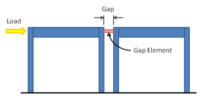
While RISA does not offer the capability to directly create a gap element, one may be indirectly created using the properties of the member and an applied thermal load. The concept is to place a ‘shrunk’ member between adjacent structures. The shrinkage of the member is achieved with a negative thermal load, in the form of a member distributed load.
The amount of shrinkage should be equal to the width of the gap, such that the structures act independently until they move close enough to each other to ‘touch’ and thereby transmit loads to each other. To calculate the thermal load required for a gap use the following formula:
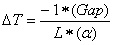
Where:
In order to prevent the gap element from ‘pulling’ its connected structures towards it due to shrinkage it must be defined as a ‘compression only’ member under the advanced options tab. It is also advisable to define the gap element as a rigid material such that the amount of load it transfers once the gap is closed is not affected by elastic shortening.
Lastly, in cases where the applied temperature would need to be of an extraordinary magnitude, it might be useful to increase the coefficient of thermal expansion of the material such that a smaller temperature load would achieve the same shrinkage.